

This tutorial will show you how to consolidate multiple worksheets into one Pivot table using Microsoft Excel.
When you create a Pivot table in Excel, you’ll usually use a list or an Excel table. For example, your collection might have different worksheets (or workbooks) with data arranged differently, but you’ll still want to create a pivot table.
Arrange your data properly, and you can easily consolidate multiple worksheets into one Pivot table. In this tutorial, we will use the consolidating sample file, which you can download from here. The workbook contains four worksheets, all of which are data collections you can use to combine into a Pivot Table.
On the “Team1” worksheet, a rectangular data region starts in cell B3 and runs down cell F7.
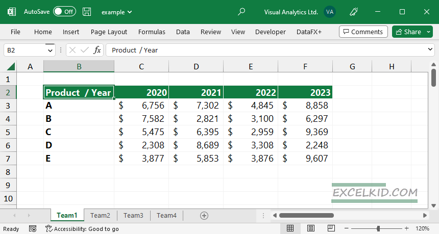
Don’t forget: your data must be in a perfect rectangle.
Here is a non-rectangular data sample. If we had Product in cell B2 and Year in cell C2, the data values would not be perfectly rectangular. In this case, the Pivot table consolidation technique would not work.
Note: We need to ensure that our data table does not have blank cells. This data summarizes yearly sales for four years (from 2020 to 2023); the years are along the top, and the row labels are along the side.
By default, the Pivot Table Wizard is not available on the ribbon.
Let us start the Pivot table wizard using a keyboard shortcut. First, press Alt+D and P to open the Pivot Table Wizard dialog box. A summary of data tables before we consolidate the worksheets: The same ranges, same shapes, and same labels are required to combine datasets into a pivot table. We will use four worksheets that contain similar data.
Select the “Team1” worksheet, and then open the Pivot Table Wizard tool to consolidate multiple worksheets into a pivot table.
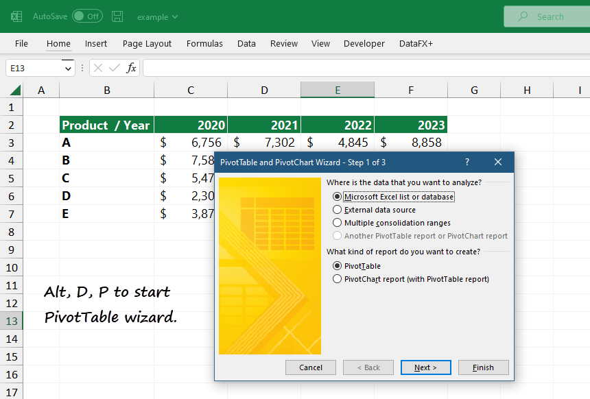
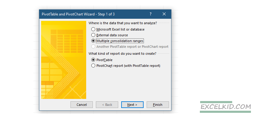
Now choose the “Multiple consolidation ranges” option under the “Where is the data that you want to analyze” section, then choose “Pivot table” and click “Next”.
Page fields are fields used to filter a Pivot Table’s contents. Locate the “How many page fields do you want” section and choose: “I will create the page fields”. Click Next.

Now, you can identify the ranges that you want to consolidate. To do that, click the collapse dialog button on the right side of the Range box.

Choose the collapse dialog button and select the first set of cells on the “Team1” worksheet. Select from B2 to F7. Next, expand the dialog box and click “Add.”
Next, click the “Team2” tab, select cells B3 to F7, expand the dialog box, and click Add. Finally, repeat these steps for the “Team3” and “Team4” worksheets.
We have identified the consolidation ranges. The next task is to specify the number of page fields we want. In this example, select 0. Click “Next” to consolidate multiple Worksheets into a new pivot table.
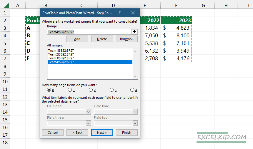
Finally, click “Finish”.

You can create an Excel table based on this data using a drill-down method. You first need to remove all field headers from the Rows and Columns area so that you are left with just the Grand Total in the Value area, so it should be a single cell, in this case, A2.
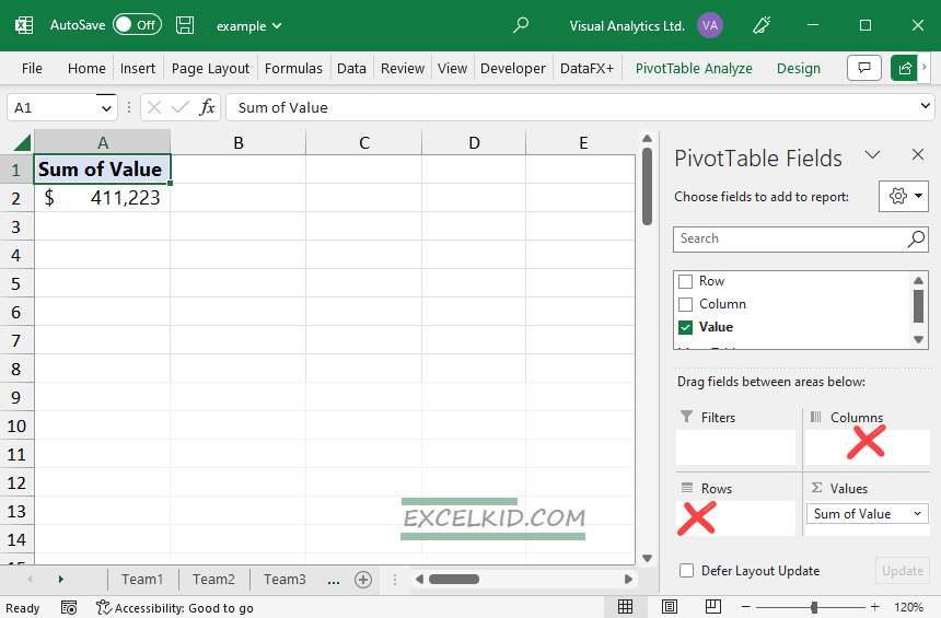
To create the Excel table, double-click that cell—in this case, cell A2. This creates an Excel table containing a list of your data, including the consolidated data.
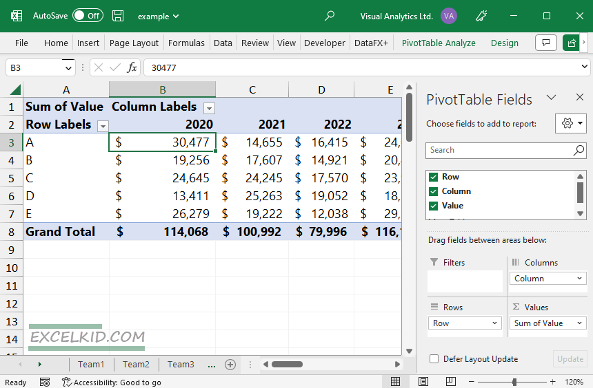
We strongly recommend using our free Excel add-in, DataXL, if you are in a hurry. It’s not complex to consolidate multiple worksheets into a Pivot table and prepare data to create dashboard templates. We have to use the same shapes for data sets. Use the drill-down method to make your life easier.